Outlier Detection

An outlier is a piece of data that deviates dramatically from the rest of the data. They might be the result of a measurement or execution mistake. Outlier analysis or outlier mining is the process of analysing outlier data.

Outlier identification, sometimes referred to as anomaly detection, is a machine learning approach that identifies data points that differ considerably from the rest of the sample. Outliers are observations that display anomalous behaviour when compared to the rest of the data and can have a substantial influence on statistical analysis and machine learning models.

Detecting Outlier

Each cluster in the K-Means clustering approach has a mean value. Objects belong to the cluster with the highest mean value. To identify the outlier, we must first set the threshold value so that any distance larger than it from the nearest cluster classifies it as an outlier for our purposes. The test data must then be distanced from each cluster mean. If the distance between the test data and the nearest cluster to it is larger than the threshold value, the test data will be classified as an outlier.

Approaches for Outlier Detection

1.Statistical Methods

Z-Score: Determines how much a data point deviates from the mean. Outliers are data points with a high absolute Z-score.
Interquartile Range (IQR): Defines a range based on the data's quartiles. Outliers are data points that fall outside of this range.

2.Distance Based Methods

Euclidean Distance: The straight-line distance between data points is measured. Outliers are data points that are far from the centre or cluster of data.
Mahalanobis Length: Accounts for fluctuating correlations and is especially beneficial for high-dimensional datasets.
DBSCAN: DBSCAN stands for Density-Based Spatial Clustering of Applications with Noise. Data points are clustered depending on their density. Outliers are points that do not fit into any of the clusters.
Local Outlier Factor (LOF): Calculates a data point's local density deviance with respect to its neighbours. Outliers are points with low local density in comparison to their neighbours.

3.Clustering-Based Methods

K-Means:Outliers might be points that do not belong to any cluster or points that belong to a tiny cluster.
Hierarchical Clustering:Small or singleton clusters in the hierarchical structure can be used to identify outliers.

4.Isolation Forest

To separate outliers, creates an ensemble of isolation trees. Outliers should have shorter pathways in the tree architectures.

5.One-Class SVM (Support Vector Machine)

Trains a model on the normal data and detects outliers, which are cases that are far from the decision border.

Steps for Outlier Detection

Data Exploration:Learn about the dataset's distribution and properties.
Feature Engineering:Select appropriate features and modifications to improve outlier detection.
Select Detection Method:Choose an appropriate outlier detection approach based on the features of the dataset and the desired sensitivity to outliers.
Set Threshold:Define a threshold over which data points are deemed outliers. The threshold used is determined on the nature of the problem.
Evaluate and Validate:Evaluate and Validate: Using relevant metrics, evaluate the performance of the outlier identification approach. Cross-validation can help guarantee generalisation.

import numpy as np
import pandas as pd
import matplotlib.pyplot as plt
import seaborn as sns
import warnings
warnings.filterwarnings("ignore")
from IPython.display import Image
from sklearn.preprocessing import StandardScaler
sns.set(style="darkgrid", palette="pastel", color_codes=True)
sns.set_context('talk')

df = pd.read_csv('insurance.csv')

df.head(5)

	age	sex	bmi	children	smoker	region	charges
0	19	female	27.900	0	yes	southwest	16884.92400
1	18	male	33.770	1	no	southeast	1725.55230
2	28	male	33.000	3	no	southeast	4449.46200
3	33	male	22.705	0	no	northwest	21984.47061
4	32	male	28.880	0	no	northwest	3866.85520

from plotly.subplots import make_subplots
import plotly.graph_objects as go

fig = make_subplots(rows=1, cols=len(df.select_dtypes(exclude='object').columns), shared_yaxes=False)
for i, col in enumerate(df.select_dtypes(exclude='object').columns):
    fig.add_trace(go.Box(y=df[col], name=col), row=1, col=i+1)

for i, col in enumerate(df.select_dtypes(exclude='object').columns):
    fig.update_xaxes(title_text=col, row=1, col=i+1)
fig.update_layout(title_text='Box Plots for Numerical Features',title_x=0.5, showlegend=False,width=1000,  height=500 )
fig.show()

def out_iqr(df , column):
    global lower,upper
    q25, q75 = np.quantile(df[column], 0.25), np.quantile(df[column], 0.75)
    iqr = q75 - q25
    cutOff = iqr * 1.5
    lower, upper = q25 - cutOff, q75 + cutOff
    print('The IQR is',iqr)
    print('The lower bound value is', lower)
    print('The upper bound value is', upper)
    df1 = df[df[column] > upper]
    df2 = df[df[column] < lower]
    return print('Total number of outliers are', df1.shape[0]+ df2.shape[0])

out_iqr(df,'age')

The IQR is 24.0
The lower bound value is -9.0
The upper bound value is 87.0
Total number of outliers are 0

import plotly.express as px
fig = make_subplots(rows=1, cols=len(df.select_dtypes(exclude='object').columns), shared_yaxes=False)
for i, col in enumerate(df.select_dtypes(exclude='object').columns):
    fig.add_trace(go.Histogram(x=df[col], name=col, ), row=1, col=i+1)
for i, col in enumerate(df.select_dtypes(exclude='object').columns):
    fig.update_xaxes(title_text=col, row=1, col=i+1)
fig.update_layout(
    title_text='Histograms for Numerical Features',
    title_x=0.5,
    showlegend=False,
    width=1000,  
    height=500  
)
fig.show()

from collections import Counter
def IQR_method(df, n, features):
    outlier_list = []
    for column in features:
        Q1 = np.percentile(df[column], 25)
        Q3 = np.percentile(df[column], 75)
        IQR = Q3 - Q1
        outlier_step = 1.5 * IQR
        outlier_list_column = df[(df[column] < Q1 - outlier_step) | (df[column] > Q3 + outlier_step)].index
        outlier_list.extend(outlier_list_column)
    outlier_list = Counter(outlier_list)
    multiple_outliers = [k for k, v in outlier_list.items() if v > n]
    total_outliers = sum(v for k, v in outlier_list.items() if v > n)
    print('Total number of outliers is:', total_outliers)
    return multiple_outliers

feature_list = ['age', 'bmi', 'children', 'charges']
Outliers_IQR = IQR_method(df, 1, feature_list)
df_out = df.drop(Outliers_IQR, axis=0).reset_index(drop=True)

Total number of outliers is: 6

features = ['age', 'bmi', 'children', 'charges']
plt.figure(figsize=(16,10))
for i, feature in enumerate(features, 1):
    plt.subplot(2, len(features), i)
    sns.histplot(df[feature], bins=30, kde=True)
    plt.title(f'{feature}  Before Dropping Outliers')
for i, feature in enumerate(features, 1):
    plt.subplot(2, len(features), i + len(features))
    sns.histplot(df_out[feature], bins=30, kde=True)
    plt.title(f'{feature}  After Dropping Outliers')
plt.tight_layout()
plt.show()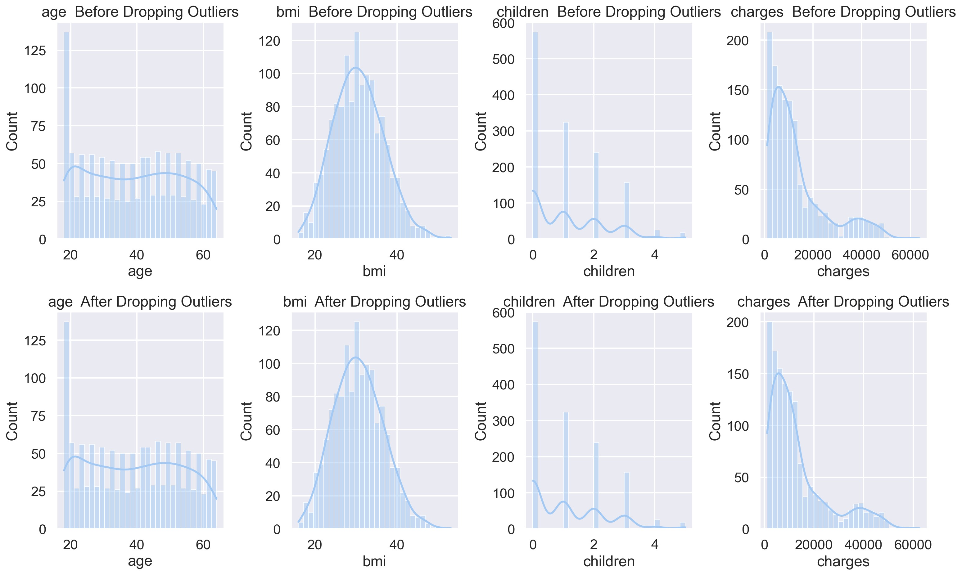

from collections import Counter
def StDev_method(df, n, features):
    outlier_indices = []
    for column in features:
        mean = df[column].mean()
        std = df[column].std()
        cutOff= std * 3
        outlier_listColumn = df[(df[column] < mean - cutOff) | (df[column] > mean +cutOff)].index
        outlier_indices.extend(outlier_listColumn)
    outlier_indices = Counter(outlier_indices)
    multiple_outliers = [k for k, v in outlier_indices.items() if v > n]
    total_outliers = sum(v for k, v in outlier_indices.items() if v > n)
    print('Total number of outliers is:', total_outliers)
    return multiple_outliers

Outliers_StDev = StDev_method(df,1,feature_list)
df_out2 = df.drop(Outliers_StDev, axis = 0).reset_index(drop=True)

Total number of outliers is: 0

data_mean, data_std = df['charges'].mean(), df['charges'].std()
cutOff = data_std * 3
lower, upper = data_mean - cutOff, data_mean + cutOff
print('The lower bound value is:', lower)
print('The upper bound value is:', upper)
plt.figure(figsize=(10, 6))
sns.histplot(x='charges', data=df, bins=70, kde=True)
plt.axvspan(xmin=lower, xmax=df['charges'].min(), alpha=0.2, color='red', label='Outlier Bound')
plt.axvspan(xmin=upper, xmax=df['charges'].max(), alpha=0.2, color='red')
plt.title('Histogram of Charges with Outlier Bound')
plt.xlabel('Charges')
plt.ylabel('Frequency')
plt.legend()
plt.show()

The lower bound value is: -23059.611444940747
The upper bound value is: 49600.45597522326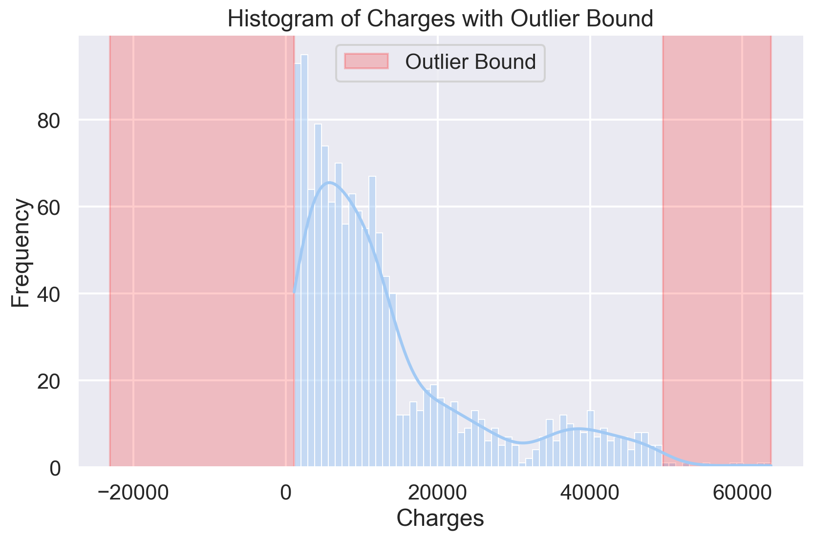

plt.figure(figsize=(16, 8))
for i, feature in enumerate(features, 1):
    plt.subplot(2, len(features), i)
    sns.scatterplot(x=range(len(df)), y=df[feature], alpha=0.5)
    plt.title(f'{feature} Before Dropping Outliers')
for i, feature in enumerate(features, 1):
    plt.subplot(2, len(features), i + len(features))
    sns.scatterplot(x=range(len(df_out2)), y=df_out2[feature], alpha=0.5)
    plt.title(f'{feature} After Dropping Outliers')
plt.tight_layout()
plt.show()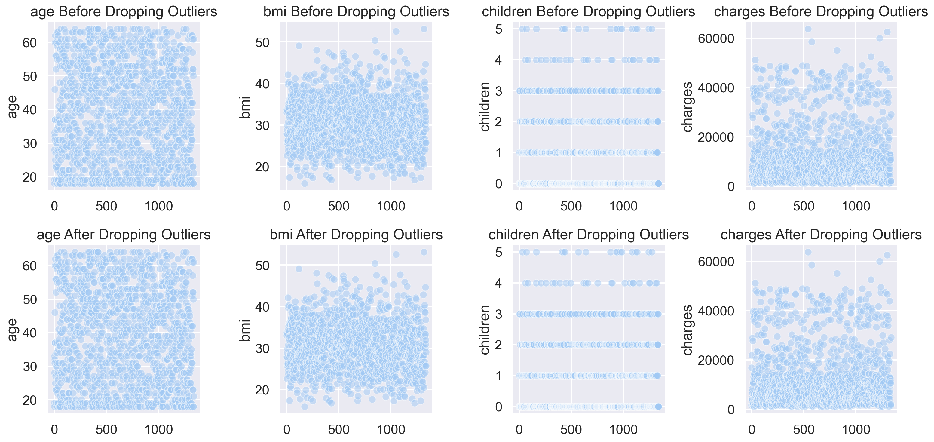

from collections import Counter
def z_score_method(df, n, features, threshold=3):
    outlier_list = []
    for column in features:
        mean = df[column].mean()
        std = df[column].std()
        zScore = abs((df[column] - mean) / std)
        outlier_list_column = df[zScore > threshold].index
        outlier_list.extend(outlier_list_column)
    outlier_list = Counter(outlier_list)
    multiple_outliers = [k for k, v in outlier_list.items() if v > n]
    total_outliers = sum(v for k, v in outlier_list.items() if v > n)
    print('Total number of outliers is:', total_outliers)
    return multiple_outliers

Outliers_z_score = z_score_method(df,1,feature_list)
df_out3 = df.drop(Outliers_z_score, axis = 0).reset_index(drop=True)

Total number of outliers is: 0

plt.figure(figsize=(16 , 10))
for i, feature in enumerate(features, 1):
    plt.subplot(3, len(features), i)
    sns.histplot(df[feature], bins=30, kde=True)
    plt.title(f'{feature} Before Dropping Outliers')
    plt.subplot(3, len(features), i + len(features))
    sns.histplot(df_out[feature], bins=30, kde=True)
    plt.title(f'{feature} After Dropping Outliers')
    plt.subplot(3, len(features), i + 2 * len(features))
    data_mean = df[feature].mean()
    data_std = df[feature].std()
    zScore = abs((df[feature] - data_mean) / data_std)
    sns.scatterplot(x=range(len(df)), y= zScore, alpha=0.5)
    plt.axhline(y=3, color='red', linestyle='--', label='Threshold')
    plt.title(f'{feature} Z-scores')
plt.tight_layout()
plt.show()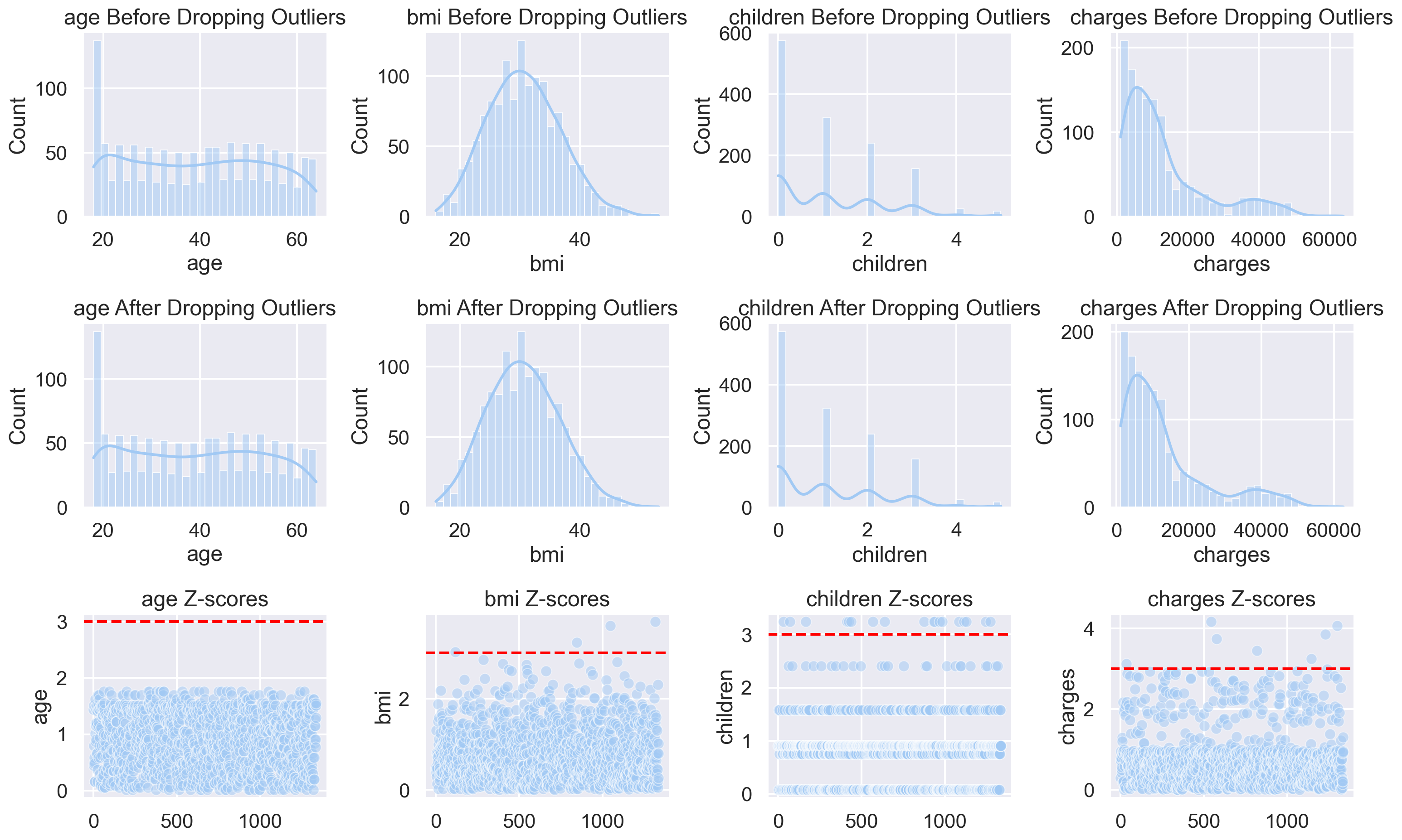

from scipy.stats import median_abs_deviation
def z_scoremod_method(df, n, features):
    outlier_list = []
    for column in features:
        data_mean = df[column].mean()
        threshold = 3
        MAD = median_abs_deviation(df[column])
        mod_z_score = abs(0.6745 * (df[column] - data_mean) / MAD)
        outlier_list_column = df[mod_z_score > threshold].index
        outlier_list.extend(outlier_list_column)
    outlier_list = Counter(outlier_list)
    multiple_outliers = [k for k, v in outlier_list.items() if v > n]
    total_outliers = sum(v for k, v in outlier_list.items() if v > n)
    print('Total number of outliers is:', total_outliers)
    return multiple_outliers

Outliers_z_score = z_scoremod_method(df,1,feature_list)
df_out4 = df.drop(Outliers_z_score, axis = 0).reset_index(drop=True)

Total number of outliers is: 2

plt.figure(figsize=(16, 12))
for i, feature in enumerate(features, 1):
    plt.subplot(3, len(features), i)
    sns.histplot(df[feature], bins=30, kde=True)
    plt.title(f'{feature} Before Dropping Outliers')
outliers_z_scoremod = z_scoremod_method(df, 1, features)
df_out_z_scoremod = df.drop(outliers_z_scoremod, axis=0).reset_index(drop=True)
for i, feature in enumerate(features, 1):
    plt.subplot(3, len(features), i + len(features))
    sns.histplot(df_out_z_scoremod[feature], bins=30, kde=True)
    plt.title(f'{feature}  Z-score Modified Method')
plt.tight_layout()
plt.show()

Total number of outliers is: 2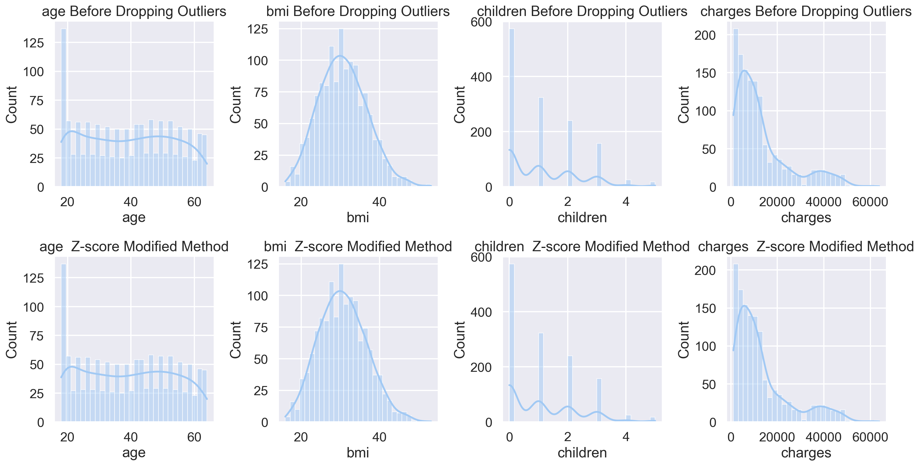

from sklearn.ensemble import IsolationForest
features = ['age', 'bmi', 'children', 'charges']
clf = IsolationForest(contamination=0.05, random_state=42)  
outliers = clf.fit_predict(df[features])
outlier_mask = outliers == -1
plt.figure(figsize=(20, 8))
for i, feature in enumerate(features, 1):
    plt.subplot(2, len(features), i)
    sns.histplot(df[feature], bins=30, kde=True)
    plt.title(f'{feature} Before Dropping Outliers')
for i, feature in enumerate(features, 1):
    plt.subplot(2, len(features), i + len(features))
    sns.scatterplot(x=range(len(df)), y=df[feature], hue=outlier_mask, palette={True: 'red', False: 'blue'})
    plt.title(f'{feature} with Outliers Highlighted')
plt.tight_layout()
plt.show()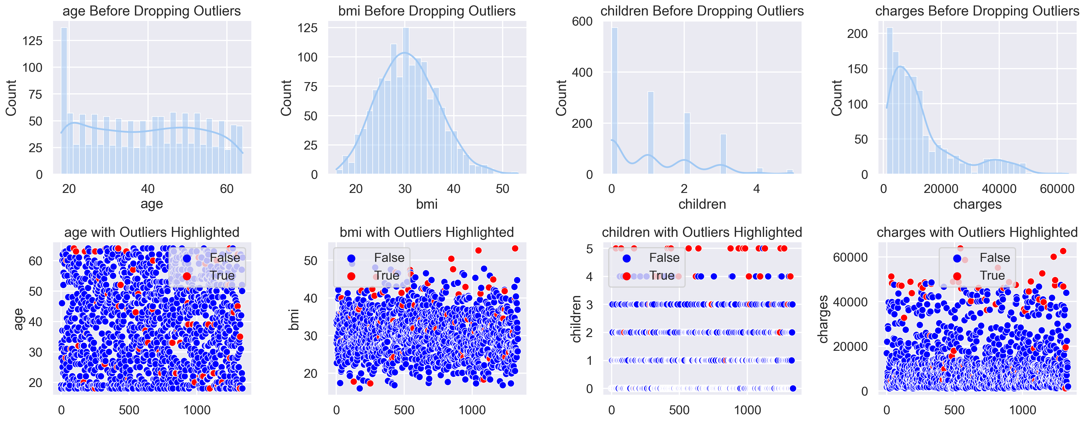

from sklearn.preprocessing import StandardScaler
from sklearn.cluster import DBSCAN
import matplotlib.pyplot as plt
import seaborn as sns
import pandas as pd
scaler = StandardScaler()
scaled_data = scaler.fit_transform(df[features])
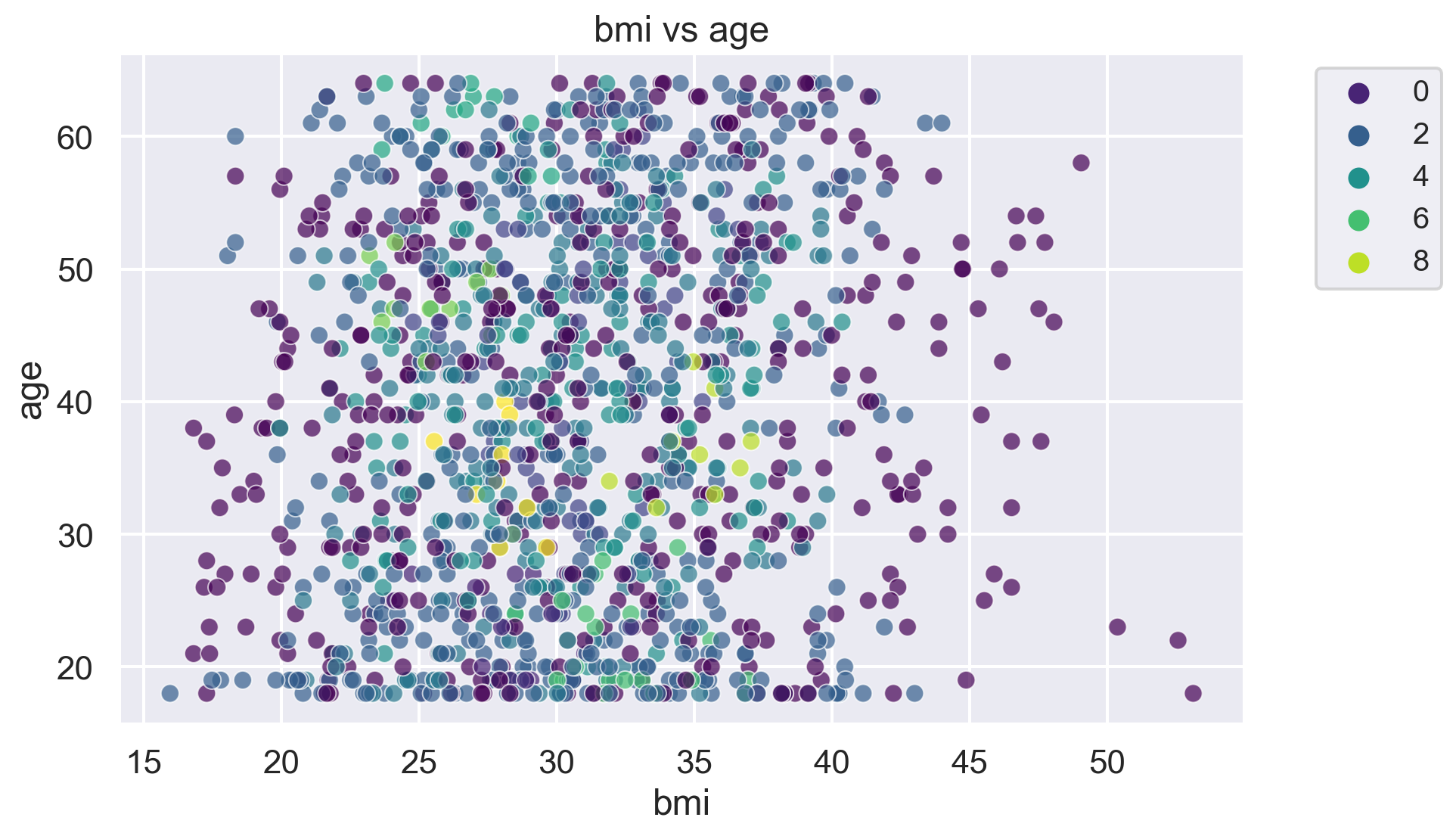
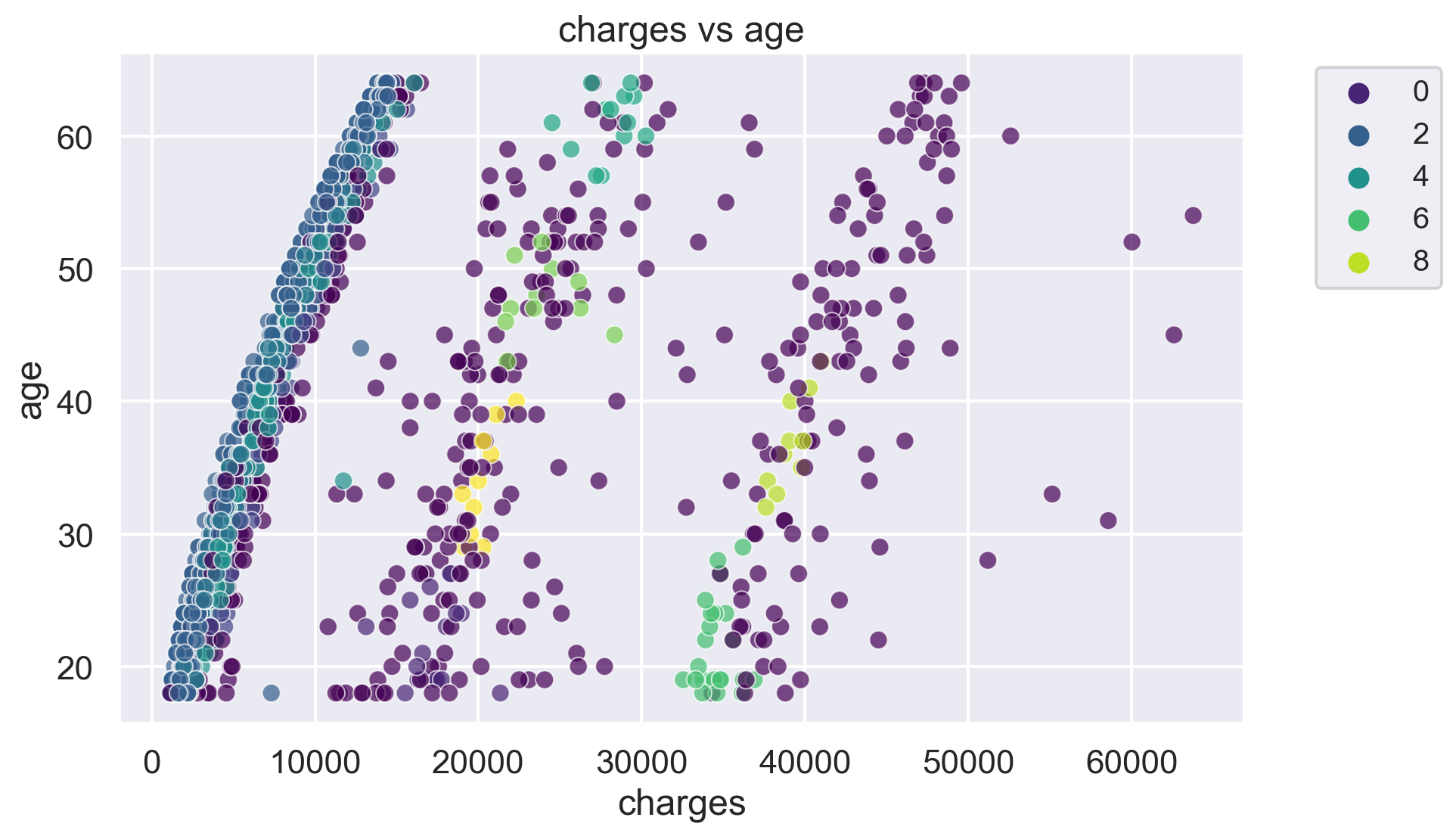
dbscan = DBSCAN(eps=0.5, min_samples=10)
label = dbscan.fit_predict(scaled_data)
nclusters = len(set(label)) - (1 if -1 in label else 0)
print('The number of clusters in the dataset is:', nclusters)
print(pd.Series(label).value_counts())
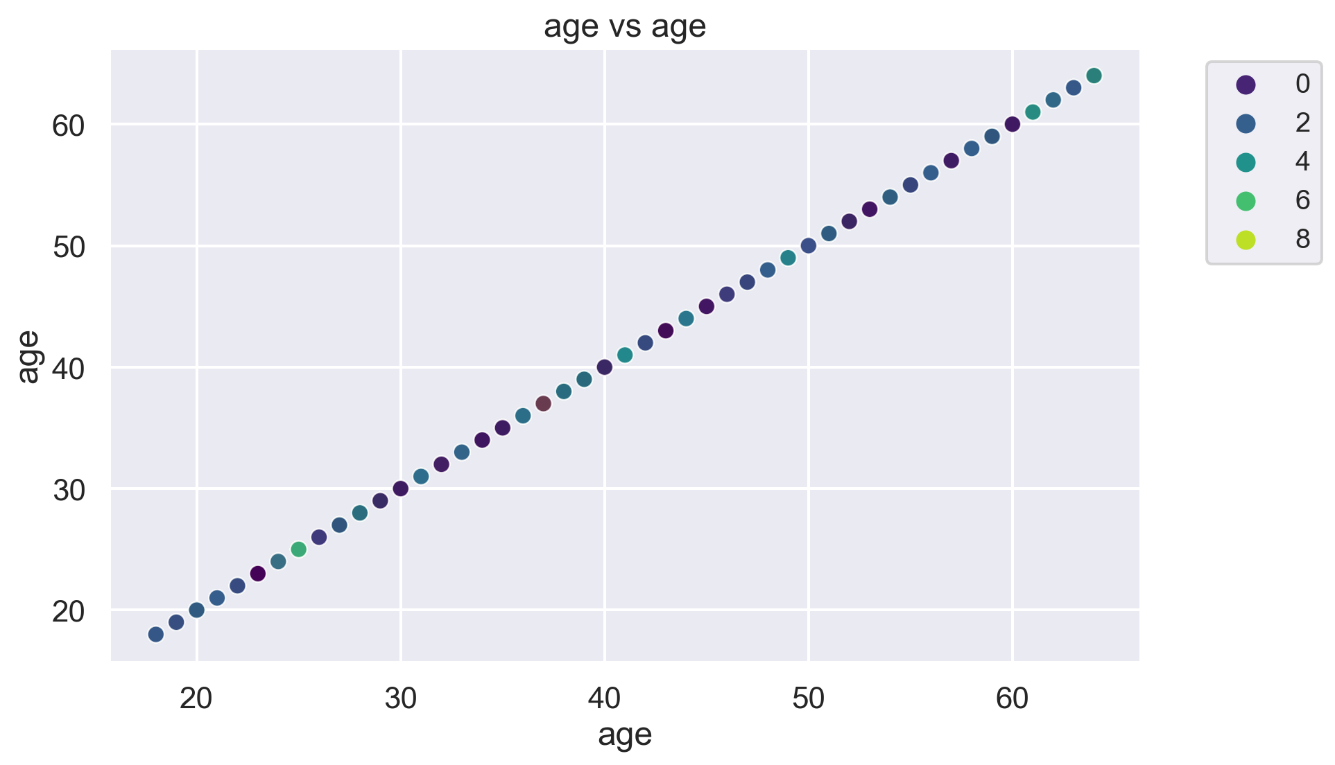
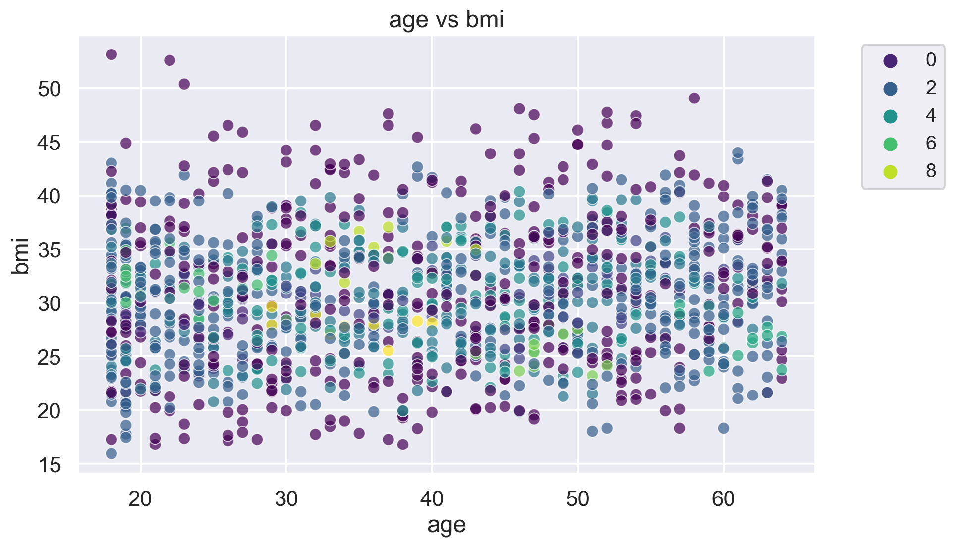
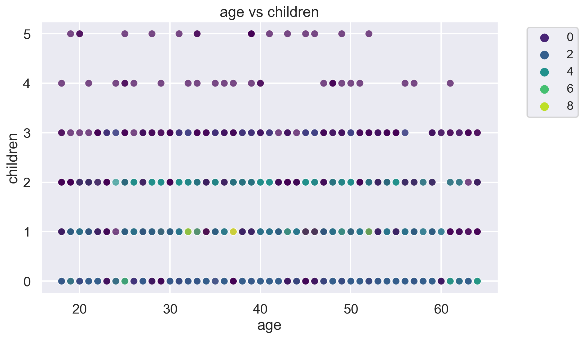
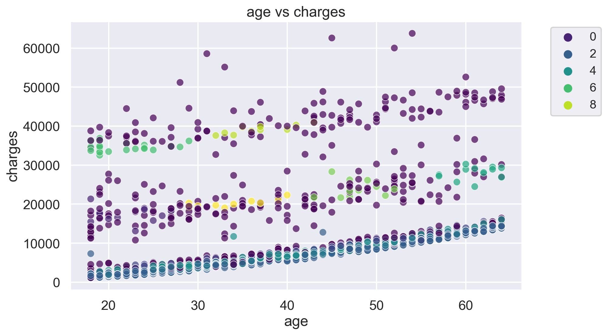
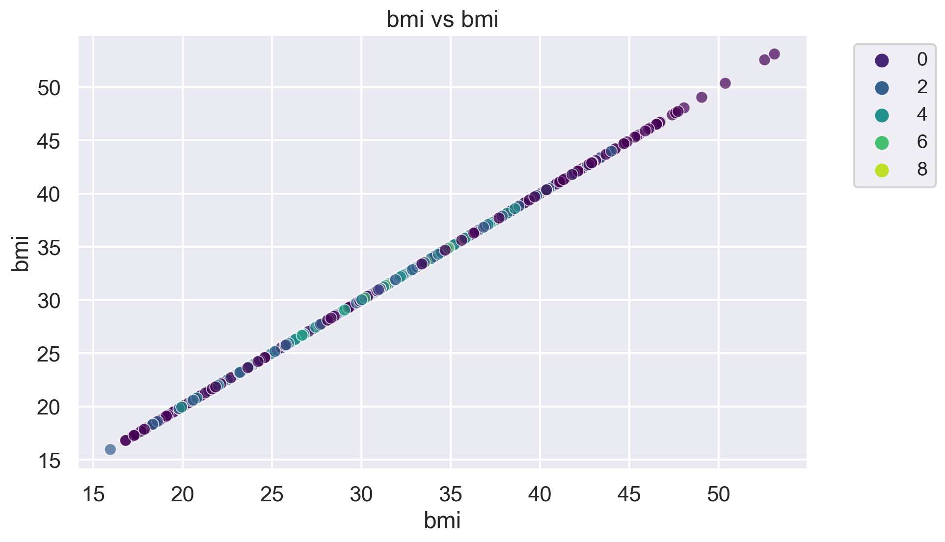
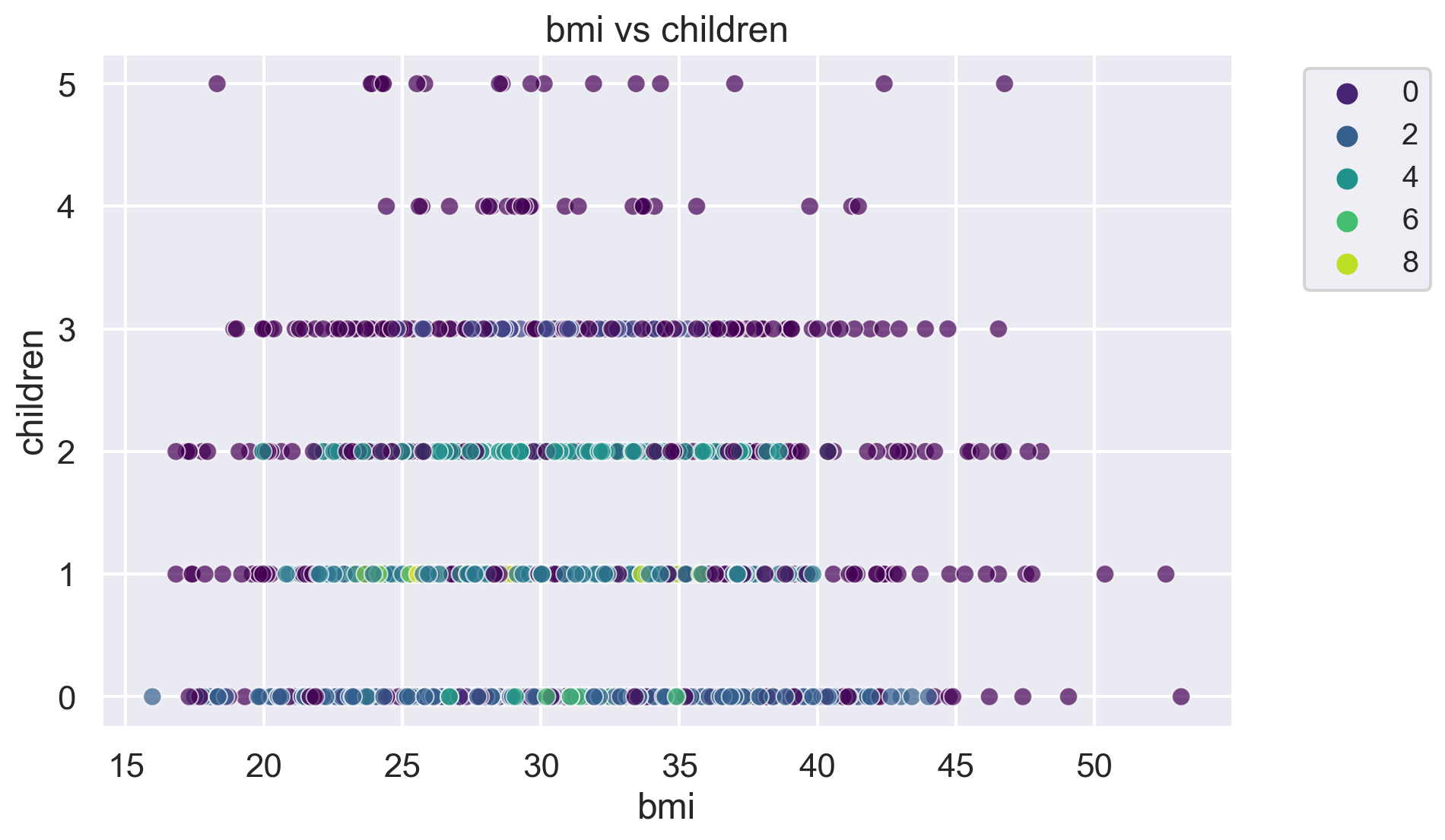
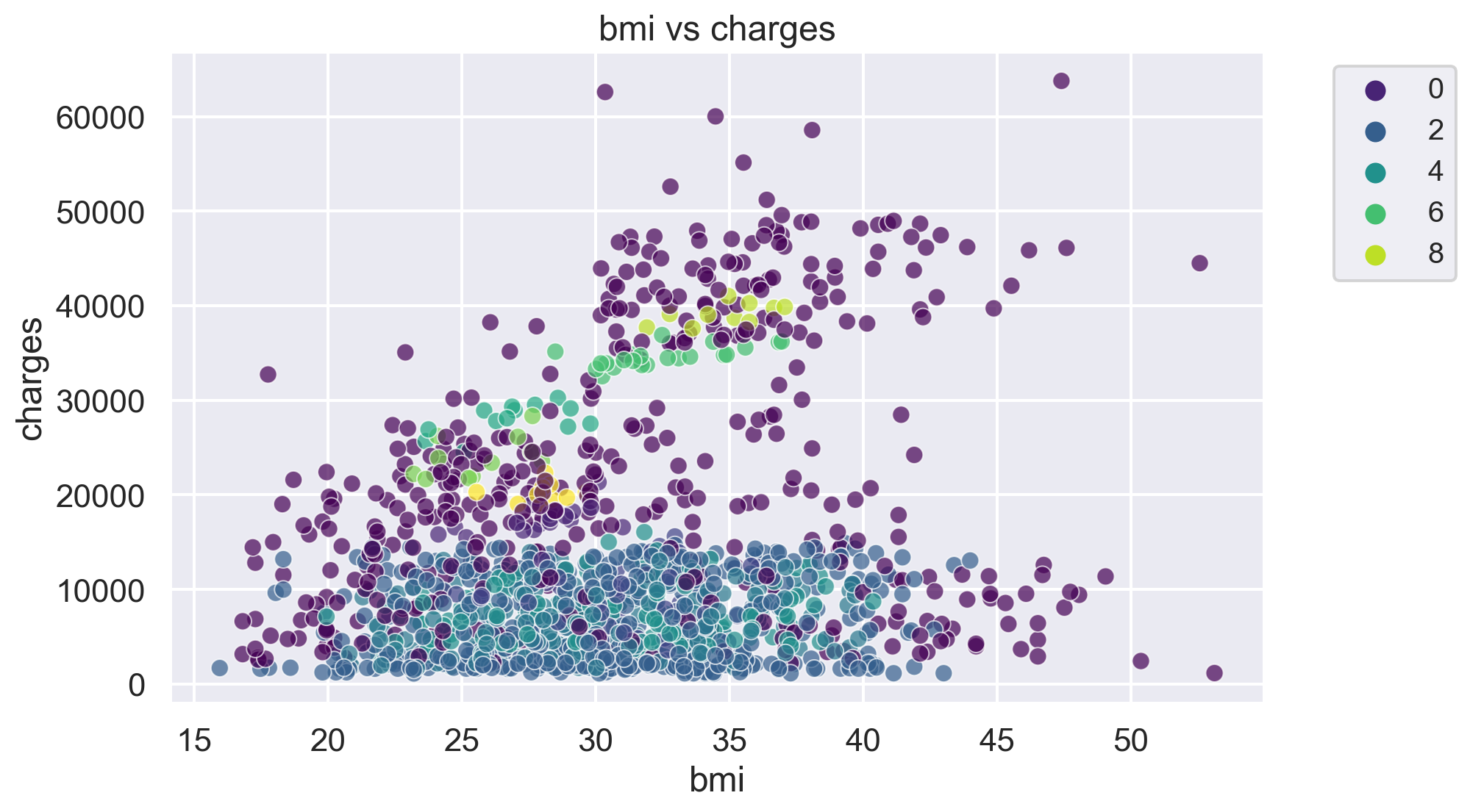
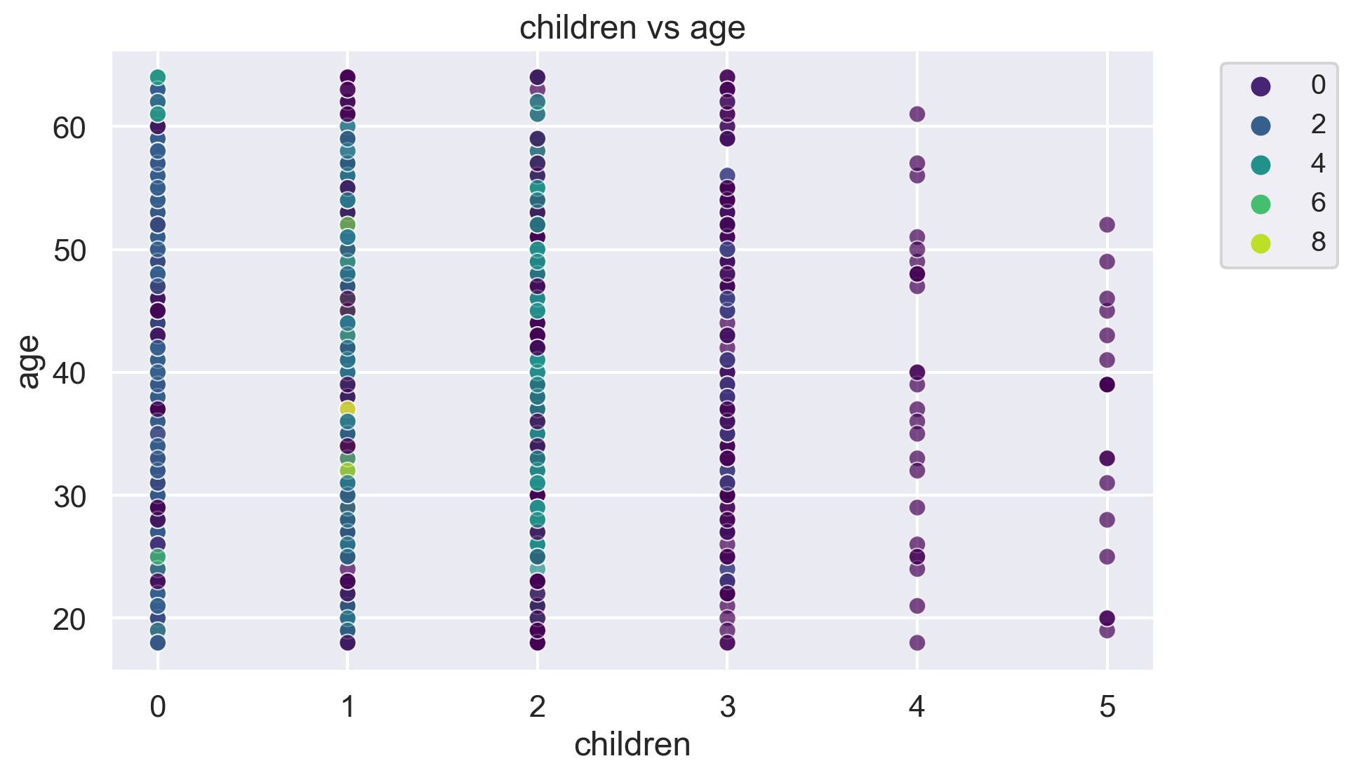
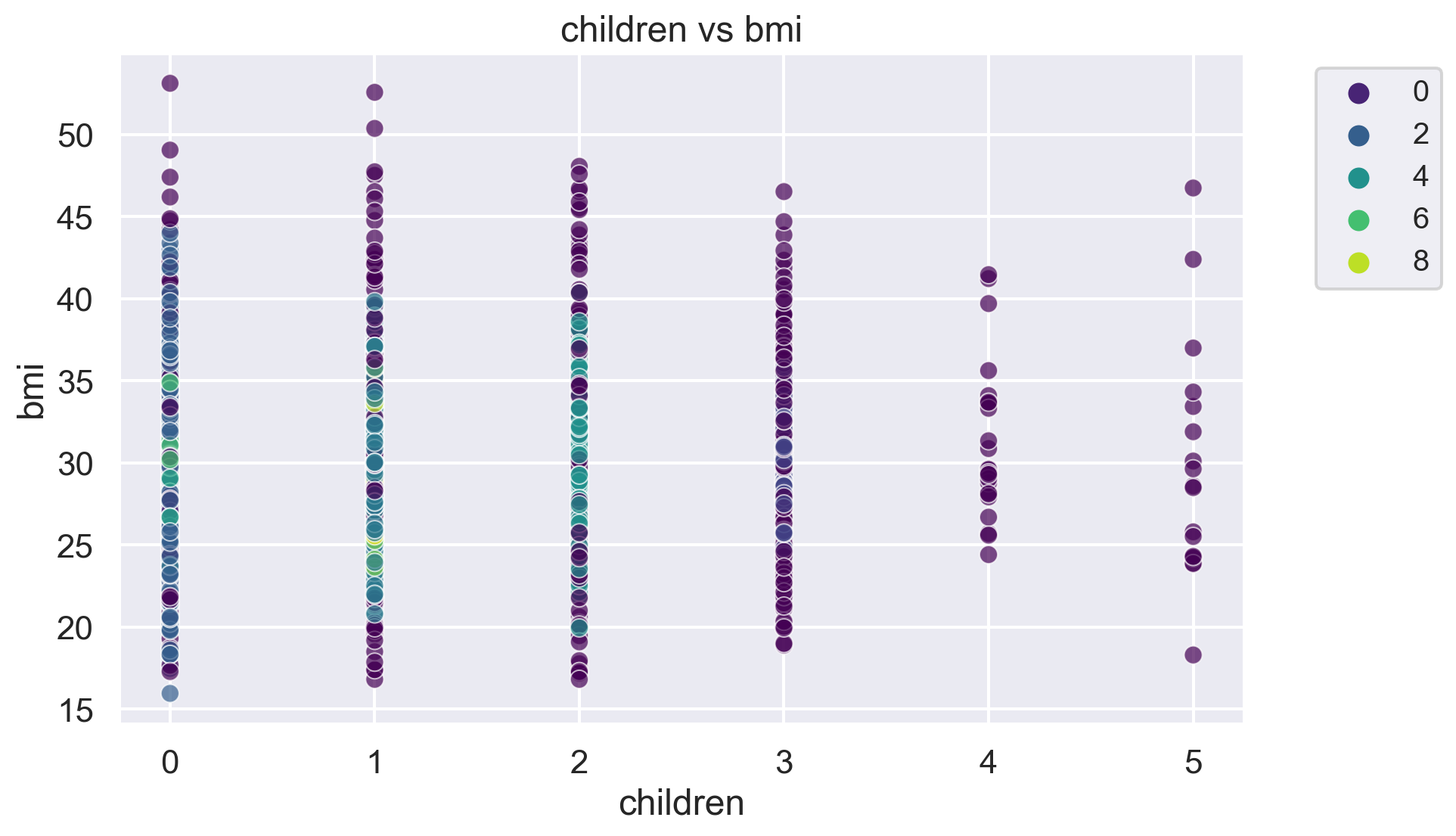
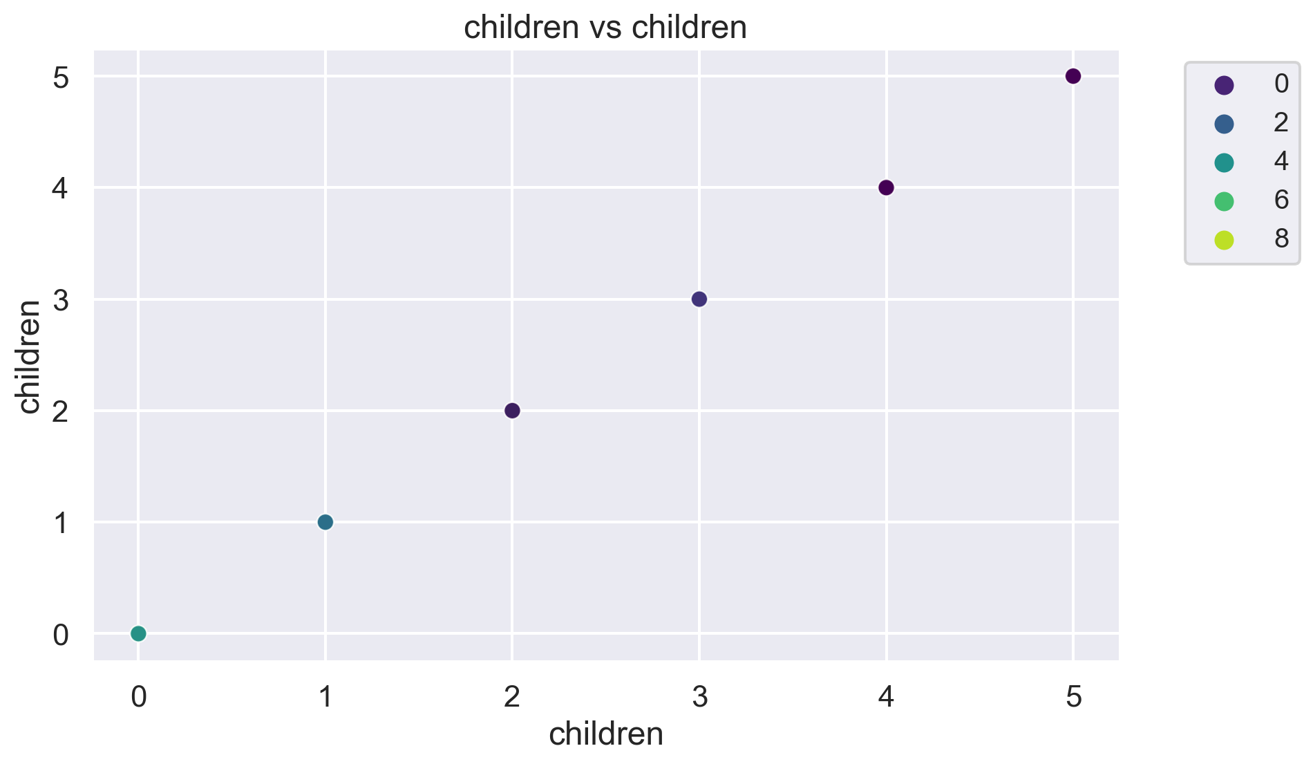
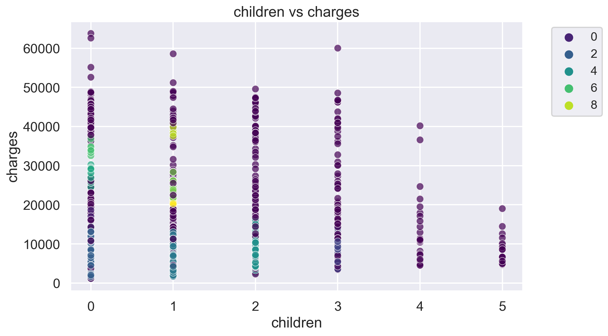
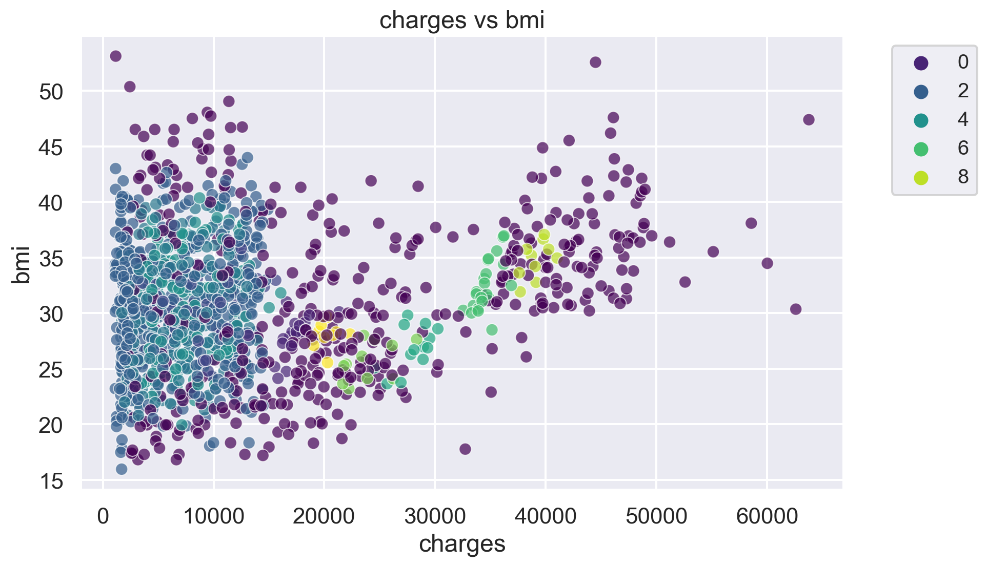
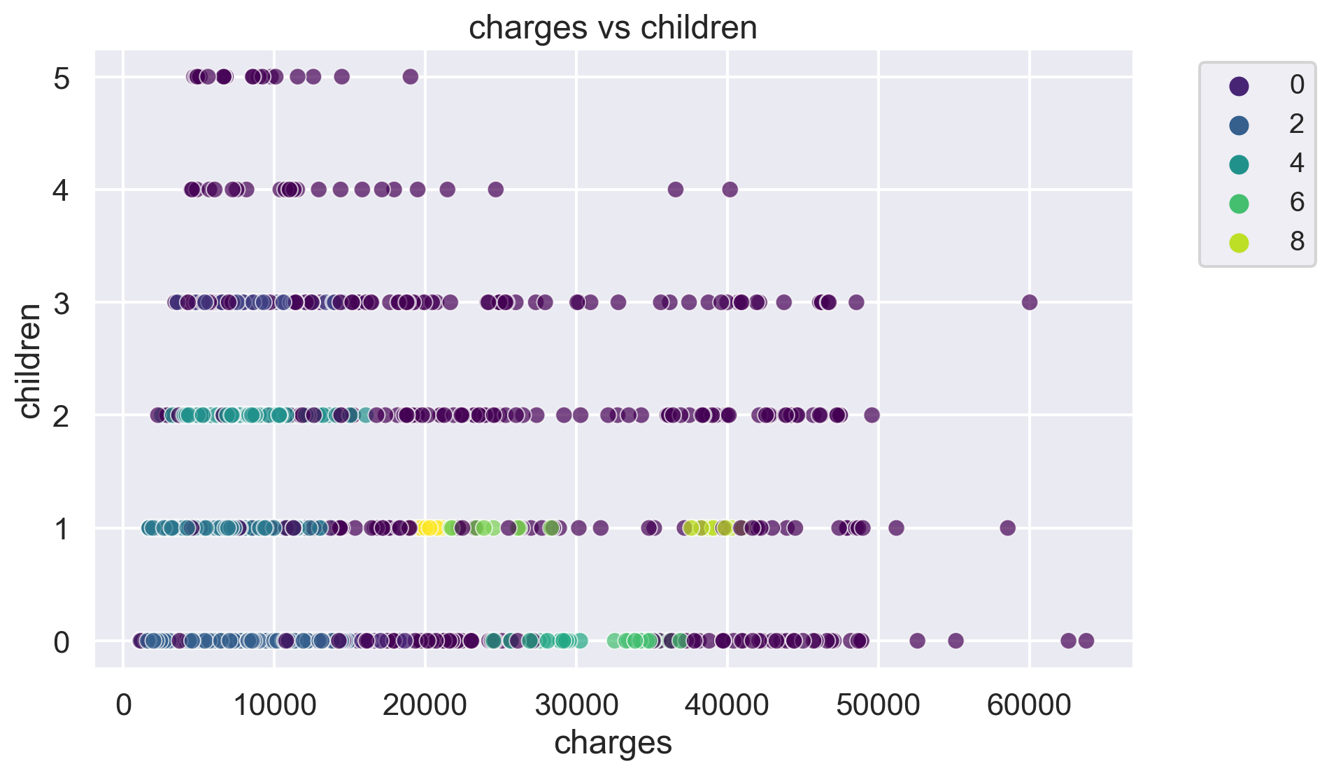
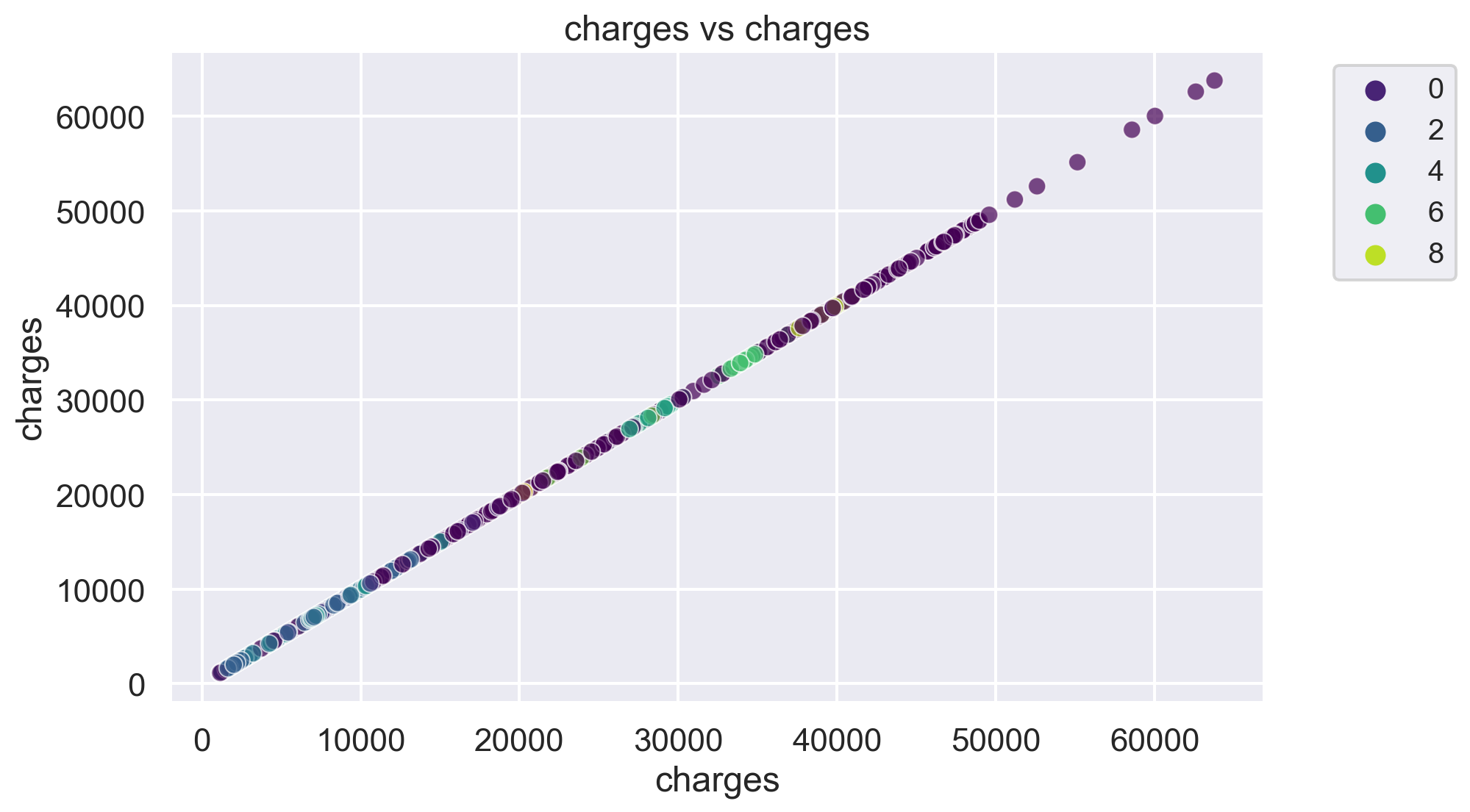
for i, feature1 in enumerate(features):
    for j, feature2 in enumerate(features):
        plt.figure(figsize=(10, 6))
        sns.scatterplot(x=df[feature1], y=df[feature2], hue=label, palette='viridis', alpha=0.7)
        plt.title(f'{feature1} vs {feature2}')
        plt.legend(fontsize="small", bbox_to_anchor=(1.05, 1), loc='upper left')
        plt.show()

The number of clusters in the dataset is: 10
-1    433
 2    417
 3    206
 4    136
 1     61
 6     22
 0     19
 5     13
 7     11
 8     10
 9     10
Name: count, dtype: int64